When we simulate data we can rely on the distribution functions like rnorm, rexp and sample from base R. However, we can also leverage the great work from authors of packages which were written to make the simulation process easier. In this blogpost I will explore some of them.
Additional packages
Before starting with the simulation packages, we can load these two packages which will help with data transformation and visualization.
wakefield
Looking for interesting packages around data simulation I stumbled across the {wakefield} package by Tyler Rinker.
Introduction can be found here. It is very easy to create data with all types of variables.
r_data_frame(
    n = 500,
    id,
    age,
    iq,
    height,
    died,
    animal,
    internet_browser,
    political
)
# A tibble: 500 x 8
   ID      Age    IQ Height Died  Animal            Browser Political
   <chr> <int> <dbl>  <dbl> <lgl> <fct>             <fct>   <fct>
 1 001      69    91     69 TRUE  Chinchilla        Chrome  Democrat
 2 002      49    87     69 FALSE Galapagos Penguin Chrome  Republican
 3 003      60   112     64 FALSE Birds Of Paradise Firefox Republican
 4 004      43    97     69 TRUE  Sea Squirt        IE      Democrat
 5 005      32    92     75 TRUE  Galapagos Penguin Chrome  Republican
 6 006      42    99     70 FALSE Ocelot            Chrome  Republican
 7 007      87    91     70 FALSE Poison Dart Frog  Chrome  Republican
 8 008      23    91     67 TRUE  Drever            Firefox Democrat
 9 009      54    94     67 FALSE Pointer           Safari  Democrat
10 010      86    96     69 TRUE  Sea Squirt        Chrome  Democrat
# ... with 490 more rows
There are a lot of predefined variables that you can use. (Call variables(type="matrix",ncols=5) to see them.)
      [,1]         [,2]          [,3]               [,4]
 [1,] "age"        "dice"        "hair"             "military"
 [2,] "animal"     "dna"         "height"           "month"
 [3,] "answer"     "dob"         "income"           "name"
 [4,] "area"       "dummy"       "internet_browser" "normal"
 [5,] "car"        "education"   "iq"               "political"
 [6,] "children"   "employment"  "language"         "race"
 [7,] "coin"       "eye"         "level"            "religion"
 [8,] "color"      "grade"       "likert"           "sat"
 [9,] "date_stamp" "grade_level" "lorem_ipsum"      "sentence"
[10,] "death"      "group"       "marital"          "sex"
      [,5]
 [1,] "sex_inclusive"
 [2,] "smokes"
 [3,] "speed"
 [4,] "state"
 [5,] "string"
 [6,] "upper"
 [7,] "valid"
 [8,] "year"
 [9,] "zip_code"
[10,]
attr(,"class")
[1] "matrix" "array"
Additionally, you can access the distribution functions easily and tweak parameters of the predefined functions.
test <- r_data_frame(
    n = 500,
    id,
    age(x=18:50),
    `Reading(mins)` = rpois(lambda=20),
    income(digits=0)
)
# A tibble: 500 x 4
   ID      Age `Reading(mins)` Income
   <chr> <int>           <int>  <dbl>
 1 001      39              22  49775
 2 002      19              25  19148
 3 003      19              20  32714
 4 004      41              19  11000
 5 005      35              21  64802
 6 006      29              20  36548
 7 007      43              21  62348
 8 008      35              18  24371
 9 009      50              18 135653
10 010      48              23  51157
# ... with 490 more rows
Looks too perfect? Include random missing values in columns 2 and 4: (Note: If you create a larger dataframe, you can use the %>% operator to structure your code better).
# A tibble: 500 x 4
   ID      Age `Reading(mins)` Income
   <chr> <int>           <int>  <dbl>
 1 001      39              22     NA
 2 002      19              25     NA
 3 003      19              20     NA
 4 004      41              19  11000
 5 005      NA              21  64802
 6 006      29              20  36548
 7 007      43              21     NA
 8 008      35              18     NA
 9 009      50              18     NA
10 010      NA              23  51157
# ... with 490 more rows
Series
{wakefield} allows us to create several variables which can be seen as a sequence, for example survey results.
r_series(likert,j = 5,n=10,name="Question")
# A tibble: 10 x 5
   Question_1    Question_2    Question_3    Question_4    Question_5
 * <ord>         <ord>         <ord>         <ord>         <ord>
 1 Strongly Dis~ Agree         Disagree      Strongly Agr~ Disagree
 2 Disagree      Strongly Dis~ Strongly Agr~ Agree         Agree
 3 Strongly Agr~ Neutral       Strongly Agr~ Strongly Agr~ Disagree
 4 Disagree      Strongly Agr~ Neutral       Strongly Agr~ Strongly A~
 5 Agree         Strongly Dis~ Agree         Strongly Dis~ Neutral
 6 Strongly Dis~ Disagree      Strongly Agr~ Strongly Agr~ Disagree
 7 Strongly Agr~ Strongly Agr~ Strongly Dis~ Strongly Agr~ Agree
 8 Strongly Agr~ Neutral       Neutral       Agree         Strongly A~
 9 Strongly Dis~ Strongly Agr~ Strongly Dis~ Neutral       Strongly A~
10 Strongly Dis~ Disagree      Disagree      Strongly Dis~ Disagree
These can also be packaged inside a data frame, for example when simulating test results for students.
r_data_frame(
  n=10,
  Student=id,
  age=rpois(14),
  r_series(grade,j=3,integer=TRUE,name="Test")
)
# A tibble: 10 x 5
   Student   age Test_1 Test_2 Test_3
   <chr>   <int>  <int>  <int>  <int>
 1 01         16     89     85     91
 2 02         17     91     87     85
 3 03         13     84     88     85
 4 04         13     91     89     83
 5 05         10     86     87     78
 6 06         15     87     87     84
 7 07         12     83     85     90
 8 08         16     89     94     84
 9 09         14     93     82     91
10 10         10     89     86     87
That is great but not very real, because the test results are completely independent from each other. The relate parameter inside the r_series function helps to connect the results, and the format is fM_sd.
- f is one of (+,-,*,/)
- M is the mean value
- sd is the standard deviation of the mean value
Examples: * additive: +3_1: The test results get better on average 3 points with a standard deviation of 1. * multiplicative: *1.05_0.2: The results get better on average 5% with a standard deviation of 0.2.
r_data_frame(
  n=10,
  Student=id,
  age=rpois(14),
  r_series(grade,j=3,integer=TRUE,name="Test",relate="+3_1")
)
# A tibble: 10 x 5
   Student   age Test_1     Test_2     Test_3
   <chr>   <int> <variable> <variable> <variable>
 1 01         13 96.6       98.8       99.6
 2 02         18 90.7       93.4       98.3
 3 03         13 83.8       88.0       92.7
 4 04         10 91.6       93.3       96.1
 5 05         15 92.3       95.5       99.6
 6 06         16 88.9       92.0       95.8
 7 07         11 93.0       96.4       98.9
 8 08         10 91.5       95.0       96.5
 9 09         14 85.9       86.5       90.3
10 10         13 84.5       88.4       90.9
With this in mind, you can create customer balances over time very easily.
balances <- r_data_frame(
  n=10,
  Client=name,
  age,
  r_series(income,j=12,name="Month",relate="*1.03_0.1")
)
This result is worth to be visualized.
balances %>%
  tidyr::pivot_longer(-c(1,2),names_to="Month") %>%
  mutate(Month=readr::parse_number(Month)) %>%
  ggplot(aes(x=Month,y=value))+geom_line()+facet_wrap(~Client,scales="free_y")
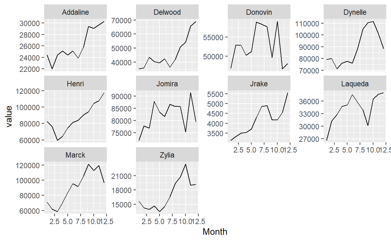
We can see that there are customers who had very positive balance development and others whose balances were fluctuating more or declining. However, when we simulate a sufficiently large number of customers, we will observe that on average the increase each month will be the desired 3% with a standard deviation of 0.1.
rcorpora
Check the github repository here.
The rcorpora library has 293 collections of words that can be very helpful for data simulation.
[1] 293 [1] "words/stopwords/de"
[2] "humans/prefixes"
[3] "humans/thirdPersonPronouns"
[4] "animals/cats"
[5] "humans/celebrities"
[6] "music/bands_that_have_opened_for_tool"
[7] "technology/knots"
[8] "foods/iba_cocktails"
[9] "words/adjs"
[10] "societies_and_groups/fraternities/professional"To view the words of one collection use the name in the corpora() function.
corpora("foods/pizzaToppings")
$description
[1] "A list of pizza toppings."

$pizzaToppings
 [1] "anchovies"        "artichoke"        "bacon"
 [4] "breakfast bacon"  "Canadian bacon"   "cheese"
 [7] "chicken"          "chili peppers"    "feta"
[10] "garlic"           "green peppers"    "grilled onions"
[13] "ground beef"      "ham"              "hot sauce"
[16] "meatballs"        "mushrooms"        "olives"
[19] "onions"           "pepperoni"        "pineapple"
[22] "sausage"          "spinach"          "sun-dried tomato"
[25] "tomatoes"
Let see how we can use this in a simulated dataframe.
tibble(
  first_name=corpora("humans/firstNames")$firstNames %>% sample(100,replace=TRUE),
  last_name=corpora("humans/lastNames")$lastNames %>% sample(100,replace=TRUE),
  self_description=corpora("humans/descriptions")$descriptions %>% sample(100,replace=TRUE),
  home_country=corpora("geography/countries")$countries %>% sample(100,replace=TRUE),
  favorite_pizza_topping=corpora("foods/pizzaToppings")$pizzaToppings %>% sample(100,replace=TRUE)
)
# A tibble: 100 x 5
   first_name last_name self_description home_country favorite_pizza_~
   <chr>      <chr>     <chr>            <chr>        <chr>
 1 Jacob      Peterson  lean             Peru         sausage
 2 Ruby       Roberts   immature         Nicaragua    Canadian bacon
 3 Carson     Gonzales  quick            Haiti        bacon
 4 Shane      Stewart   one-sided        Nauru        ground beef
 5 Molly      Rice      civil            Iraq         breakfast bacon
 6 Stephanie  Chavez    ambitious        Monaco       green peppers
 7 Kaden      Gutierrez picky            Egypt        Canadian bacon
 8 Valerie    Foster    irritating       Malta        spinach
 9 Genesis    Owens     talented         Tuvalu       green peppers
10 Amy        Wood      unfriendly       Vatican Cit~ hot sauce
# ... with 90 more rows
charlatan
Similar to wakefield, charlatan has some out-of-the-box variables that can be used in your simulated data.
 [1] "Development worker, community"
 [2] "Veterinary surgeon"
 [3] "Advertising account executive"
 [4] "Optician, dispensing"
 [5] "Museum education officer"
 [6] "Research officer, trade union"
 [7] "Engineer, automotive"
 [8] "Pharmacist, community"
 [9] "Sales promotion account executive"
[10] "Customer service manager"
You can even use get typical names or jobs for a given country. To see the available languages and countries type charlatan::PersonProvider$new()$allowed_locales().
ch_name(n=10,locale="de_DE")
 [1] "Ernestine Drubin"             "Burkhardt Koch B.Sc."
 [3] "Christof Barth B.Eng."        "Univ.Prof. Burkhardt Beier"
 [5] "Lambert Mans-Bolnbach"        "Prof. Darius Anders B.Sc."
 [7] "Univ.Prof. Felix Römer B.Sc." "Kay-Uwe Atzler-Döhn"
[9] "Reingard Neuschäfer B.Eng." "Klaus-Dieter Hölzenbecher" ch_phone_number(locale="de_DE",n=10)
[1] "+49(0)7367 624040" "03154789561" "(08044) 075665"
[4] "(02605) 71714" "+49(0)6273434607" "06457 409315"
[7] "00114 07336" "+49(0)6680 38728" "04223885899"
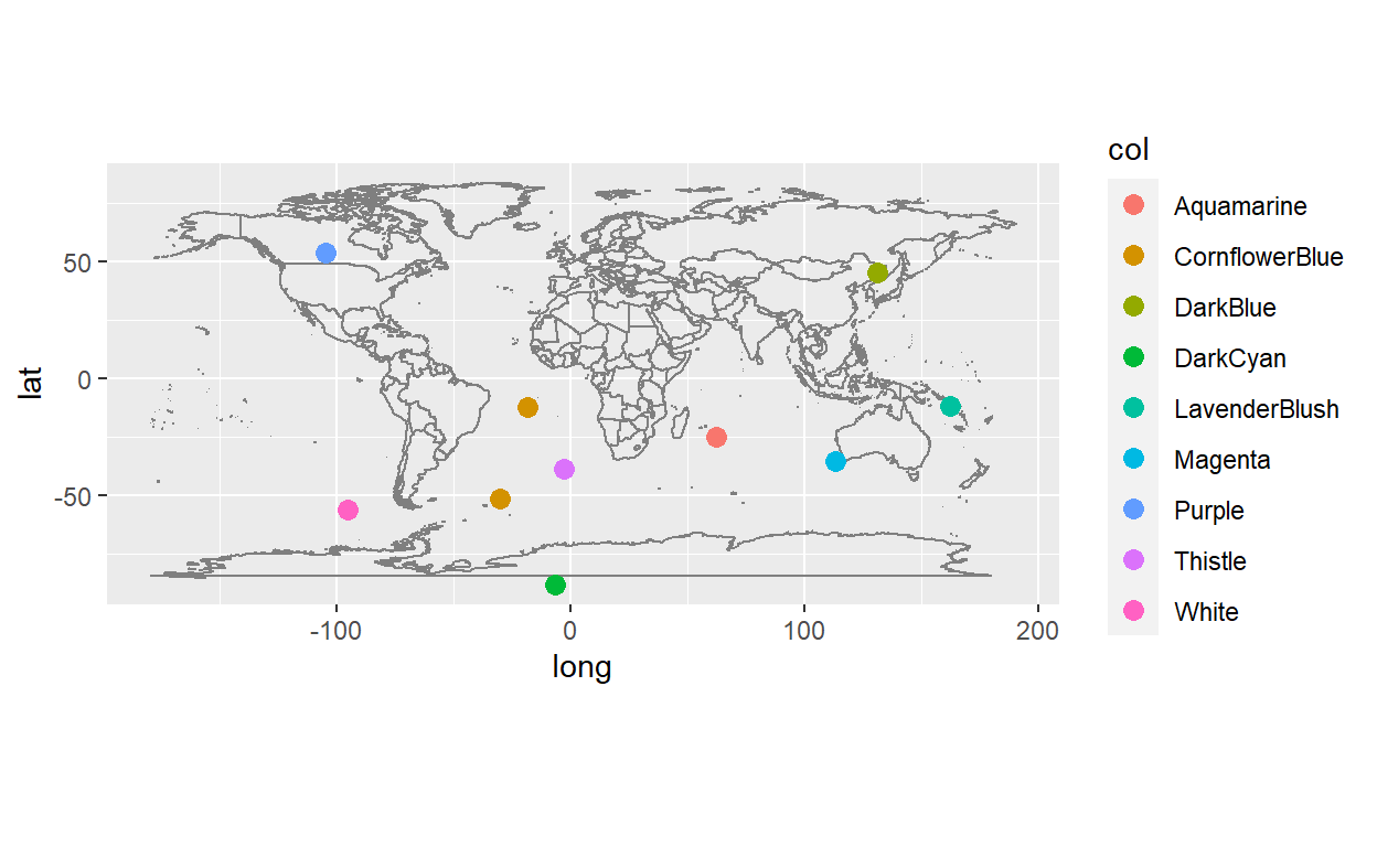
[10] "+49 (0) 4533 749527"A nice small application with fake locations and random R colors.
locations <- data.frame(lon=ch_lon(n=10),lat=ch_lat(n=10),col=ch_color_name(n=10))

ggplot(locations)+
  borders("world")+
  geom_point(aes(x=lon,y=lat,col=col),size=3)+
  coord_quickmap()
fabricatr
Easy creation of hierarchical data is possible with {fabricatr}. In this example there are five families, each one has between 1 and 12 members. Each family member has between 1 and 5 accounts. With add_level() we can automatically produce a table that shows all accounts of all members in all families.
library(fabricatr)

fabricate(
  family  = add_level(N = 5,
  n_members = sample(1:12, N, replace = TRUE,prob=12:1)),

  members  = add_level(N = n_members,
  n_accounts = sample(1:5,N,replace=TRUE,prob=(5:1)^2)),

  account = add_level(N = n_accounts)
  ) %>%
head(10)
   family n_members members n_accounts account
1       1         2      01          2      01
2       1         2      01          2      02
3       1         2      02          1      03
4       2         9      03          4      04
5       2         9      03          4      05
6       2         9      03          4      06
7       2         9      03          4      07
8       2         9      04          2      08
9       2         9      04          2      09
10      2         9      05          2      10
Link levels. We can create 15 clients with their birth year and join year and some correlation between both variables.
df <- fabricate(
  age = add_level(N=51, birth_year=1950:2000),
  tenure = add_level(N = 20, join_year=1991:2010, nest = FALSE),
  client = link_levels(N = 15, by = join(age, tenure, rho = 0.7))
)

df %>% select(client,birth_year,join_year)
   client birth_year join_year
1      01       1971      1998
2      02       1999      2009
3      03       1989      2006
4      04       1973      2008
5      05       1978      1996
6      06       1983      2001
7      07       1960      1996
8      08       1978      1997
9      09       1975      1997
10     10       1984      2002
11     11       1997      2008
12     12       1991      2002
13     13       1963      1999
14     14       1996      2009
15     15       1984      2001
Ordered data
fabricatr has an amazing function to create ordered categorical data.
The function we need is draw_ordered. It internally simulates a numeric variable (x) and breaks them into predefined categories.
draw_ordered(
  x = rnorm(10),
  breaks = c(-2,-1,0.8,2),
  break_labels = c("Very boring","Boring","OK","Interesting","Very Interesting")
)
 [1] OK          Boring      OK          Interesting OK
 [6] Boring      OK          OK          Interesting Interesting
Levels: Very boring Boring OK Interesting Very Interesting
Let’s take a look at another example where we have two types of clients, gold clients that receive a yearly gift from the bank and standard clients that do not. How could we simulate their responses to a satisfaction survey?
df <- fabricate(
  N = 100,
  gold_client_flag = draw_binary(prob = 0.3, N),
  satisfaction = draw_ordered(
    x = rnorm(N, mean = -0.4 + 1.2 * gold_client_flag),
    breaks = c(-1.5, -0.5, 0.5, 1.5),
    break_labels = c("Very Unsatisfied", "Unsatisfied", "Neutral",
                     "Satisfied", "Very Satisfied")
  )
)
   ID gold_client_flag     satisfaction
1 001                0 Very Unsatisfied
2 002                0          Neutral
3 003                0          Neutral
4 004                0        Satisfied
5 005                0      Unsatisfied
6 006                0          Neutral
We can summarize the results and see the differences between the two groups. Ideal data for teaching hypothesis testing.
df %>% count(gold_client_flag,satisfaction) %>%
  tidyr::pivot_wider(id_cols=satisfaction,names_from="gold_client_flag",values_from="n")
# A tibble: 5 x 3
  satisfaction       `0`   `1`
  <fct>            <int> <int>
1 Very Unsatisfied    12    NA
2 Unsatisfied         22     2
3 Neutral             29     9
4 Satisfied           11     9
5 Very Satisfied       1     5
Time series
Example from this article.
This example contains the GDP of five countries over the course of five years.
panel_units <- fabricate(
  countries = add_level(
    N = 5,
    base_gdp = runif(N, 15, 22),
    growth_units = runif(N, 0.2, 0.8),
    growth_error = runif(N, 0.1, 0.5)
  ),
  years = add_level(
    N = 5,
    ts_year = 0:4,
    gdp_measure = base_gdp + (ts_year * growth_units) + rnorm(N, sd=growth_error)
  )
)

head(panel_units,10)
   countries base_gdp growth_units growth_error years ts_year
1          1 15.81650    0.2936397    0.2843482    01       0
2          1 15.81650    0.2936397    0.2843482    02       1
3          1 15.81650    0.2936397    0.2843482    03       2
4          1 15.81650    0.2936397    0.2843482    04       3
5          1 15.81650    0.2936397    0.2843482    05       4
6          2 15.25248    0.5143369    0.4467515    06       0
7          2 15.25248    0.5143369    0.4467515    07       1
8          2 15.25248    0.5143369    0.4467515    08       2
9          2 15.25248    0.5143369    0.4467515    09       3
10         2 15.25248    0.5143369    0.4467515    10       4
   gdp_measure
1     15.54446
2     16.25074
3     16.26999
4     16.50294
5     17.46510
6     15.13692
7     16.36070
8     16.30388
9     16.94710
10    17.80540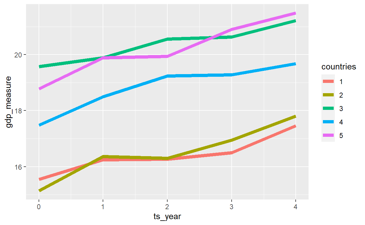
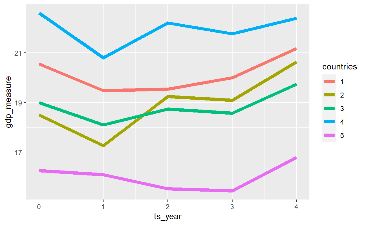
We can take this to the next level and introduce some year specific information and then cross this with the country specific information. We just have to add one layer.
panel_global_data <- fabricate(
  years = add_level(
    N = 5,
    ts_year = 0:4,
    year_shock = rnorm(N, 0, 0.5) #each year has a global trend
  ),
  countries = add_level(
    N = 5,
    base_gdp = runif(N, 15, 22),
    growth_units = runif(N, 0.2, 0.5),
    growth_error = runif(N, 0.1, 0.5),
    nest = FALSE
  ),
  country_years = cross_levels(
    by = join(years, countries),
    gdp_measure = base_gdp + year_shock + (ts_year * growth_units) +
      rnorm(N, sd=growth_error)
  )
)
GenOrd
This package helps to create discrete random variables with prescribed correlation matrix and marginal distributions.
library(GenOrd)


k <- 4 #number of random variables
marginal <- list(0.6, c(1/3,2/3), c(1/4,2/4,3/4), c(1/5,2/5,3/5,4/5))
Read the list as follows:
- We will create 4 random variables.
- The first variable will have two values: 60% of the data will be 1, 40% will be 2.
- The second variable will have three values, 1,2 and 3 with a probability of 33% each.
- etc…
- Each vector in this list refers to one variable, and we will see the cumulative probability for each value.
corrcheck(marginal)
[[1]]
4 x 4 Matrix of class "dsyMatrix"
           [,1]       [,2]       [,3]       [,4]
[1,]  1.0000000 -0.8333333 -0.8215838 -0.8660254
[2,] -0.8333333  1.0000000 -0.9128709 -0.9237604
[3,] -0.8215838 -0.9128709  1.0000000 -0.9486833
[4,] -0.8660254 -0.9237604 -0.9486833  1.0000000

[[2]]
4 x 4 Matrix of class "dsyMatrix"
          [,1]      [,2]      [,3]      [,4]
[1,] 1.0000000 0.8333333 0.8215838 0.8660254
[2,] 0.8333333 1.0000000 0.9128709 0.9237604
[3,] 0.8215838 0.9128709 1.0000000 0.9486833
[4,] 0.8660254 0.9237604 0.9486833 1.0000000
This function shows what are allowable ranges for the correlation matrix, given the input from the marginal distributions.
We will create 1000 observations, with the given correlation matrix. Each variable will have the marginal distribution described above.
n <- 1000 # sample size
m <- ordsample(n, marginal, Sigma)

df <- data.frame(m)
head(df)
  X1 X2 X3 X4
1  1  1  4  1
2  2  3  4  5
3  1  2  2  3
4  2  3  3  4
5  2  3  3  5
6  2  3  4  5
Let’s verify that the data is actually what we expected. We check the correlation and the marginal distribution for two of the variables.
cor(df)
          X1        X2        X3        X4
X1 1.0000000 0.4894198 0.3312862 0.2572479
X2 0.4894198 1.0000000 0.4567171 0.3850669
X3 0.3312862 0.4567171 1.0000000 0.4893278
X4 0.2572479 0.3850669 0.4893278 1.0000000
df %>% count(X4)
  X4   n
1  1 182
2  2 193
3  3 218
4  4 212
5  5 195
df %>% count(X1)
  X1   n
1  1 584
2  2 416
Later we can rename the columns and values, but will have assured that they have the desired correlations.
More packages
In this blogpost by Joseph Rickert on R Views.