In this article I want to show how the rmultinom() function can help to simulate data. We will simulate client data, and for each client we will create transactions.
The rmultinom() function simulates the multinomial distribution (Link).
rmultinom - like a game setup
In my head I always picture the multinomial distribution as a game setup. You have N balls and K bins. Instead of the number of bins, we send a vector of probabilities (of length K), how likely it is for the balls to land in each bin (you can imagine that some bins are closer and others are further away, or that some are larger than others). This vector will be normalized automatically, so you do not have to worry about this.
Let’s try an example, with N=1000 and K=5. We want one of the bins to be twice as large as the others.
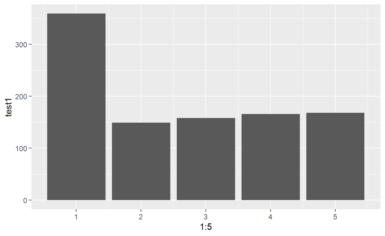
An application of rmultinom
How can we use this function to create transactions for a given number of customers? The key is to simulate all important values on client level and use rmultinom to decompose the values into smaller portions. First, let’s get some clients.
set.seed(61)

age <- rnorm(10,mean=50,sd=15) %>% pmax(18) %>% round()
tenure <- (age - 18 - runif(10,1,30)) %>% pmax(0) %>% round()
income <- rexp(10,0.0001) %>% round(2)

client <- data.frame(id=1:10,age,tenure,income)

client
   id age tenure   income
1   1  44     22 32181.33
2   2  44      7  5454.56
3   3  24      3  4559.78
4   4  55     34 26790.03
5   5  29      0 18592.27
6   6  47     19 40229.93
7   7  61     14  1065.49
8   8  58     17  2750.75
9   9  71     49 12292.53
10 10  45     15   282.05
For this exercise, we do not distinguish between different types of transactions. In practice, it would make sense to separate rent, supermarket, transport and other categories.
We create a second dataframe for clients, which contains “invisible” information needed for the transactions. Let’s begin with the total spending. This can depend on anything we know about the client. In this case, we will assume that each client has more or less the same behavior and spends around 70% of their income. The standard deviation of 0.1 assures that this value varies from client to client.
cl_secret_info <- client

cl_secret_info$total_spend <- (cl_secret_info$income * rnorm(10,0.7,sd=0.1)) %>% round(2)

cl_secret_info
   id age tenure   income total_spend
1   1  44     22 32181.33    20755.16
2   2  44      7  5454.56     4342.34
3   3  24      3  4559.78     3280.65
4   4  55     34 26790.03    21012.47
5   5  29      0 18592.27    13990.48
6   6  47     19 40229.93    25986.32
7   7  61     14  1065.49      699.14
8   8  58     17  2750.75     2158.39
9   9  71     49 12292.53    10135.33
10 10  45     15   282.05      160.08
The next ingredient is the number of transactions. For this example, we create a formula depending on age: Clients which are younger than 50 have (on average) a higher number of transactions per month.
cl_secret_info$n_trans <- ifelse(cl_secret_info$age < 50, rbinom(10,60,0.5),rbinom(10,60,0.3))

cl_secret_info
   id age tenure   income total_spend n_trans
1   1  44     22 32181.33    20755.16      27
2   2  44      7  5454.56     4342.34      37
3   3  24      3  4559.78     3280.65      28
4   4  55     34 26790.03    21012.47      25
5   5  29      0 18592.27    13990.48      32
6   6  47     19 40229.93    25986.32      27
7   7  61     14  1065.49      699.14      11
8   8  58     17  2750.75     2158.39      14
9   9  71     49 12292.53    10135.33      16
10 10  45     15   282.05      160.08      27
Now we already know that our transaction table will have 244 rows, the sum of all our 10 clients’ transactions.
We will create a last parameter which is an indicator of how similar the transactions are. You could split $100 into one large transaction of $80 and four small transactions of $5 each or you could have five transactions of around $20 each. The higher the value of diff_trans the higher the variability within the transactions of a client.
   id age tenure   income total_spend n_trans diff_trans
1   1  44     22 32181.33    20755.16      27        328
2   2  44      7  5454.56     4342.34      37         55
3   3  24      3  4559.78     3280.65      28         38
4   4  55     34 26790.03    21012.47      25         65
5   5  29      0 18592.27    13990.48      32          1
6   6  47     19 40229.93    25986.32      27       1408
7   7  61     14  1065.49      699.14      11          1
8   8  58     17  2750.75     2158.39      14         47
9   9  71     49 12292.53    10135.33      16        183
10 10  45     15   282.05      160.08      27          2
Now we have all the necessary ingredients to split total_spend into n_trans transactions for each client. And this is the moment where the rmultinom function is extremely helpful. Let’s take a look at the first client, who spends $20755.16 in 27 transactions. The high diff_trans value indicates that there will likely be some very high transaction values and some very low.
Before doing the rmultinom magic, we will create the vector with the bins first. Remember that this vector determines how “large” each bin is or how likely it is to
bins <- runif(cl_secret_info$n_trans[1],min=1,max=cl_secret_info$diff_trans[1])

transactions1 <- rmultinom(1,cl_secret_info$total_spend[1],bins)

df <- data.frame(client_id=1, trans_id=1:cl_secret_info$n_trans[1],value=transactions1)
Automate this for all customers
In order to efficiently do this for all customers we will put what we just did in a function.
create_transactions <- function(i) {
  bins <- runif(cl_secret_info$n_trans[i],min=1,max=cl_secret_info$diff_trans[i])

  transactions <- rmultinom(1,cl_secret_info$total_spend[i],bins)

  df <- data.frame(client_id=i, trans_id=1:cl_secret_info$n_trans[i],value=transactions)

  return(df)
}
We call this function repeatedly with lapply.
Finally, we bind all the transactions from all clients together in our final dataframe.
trans_df <- do.call(rbind,trans_list)
Other possible applications
- Students and grades (it is easier if the grades are points and you have a total number of points to reach). You might want to check the package {wakefield} to create sequences of grades / tests etc.
- Products and sales numbers in supermarkets.
- Animals and tracked kilometers.