Packages
Most of the functions that we are using here are part of base R.
We will need some functions from the {dplyr} and {ggplot2} packages for quick visualizations, but these are optional.
Data simulation
In this post we will learn how to simulate data like this:
  client_id    name age  ocupation balance married_flg
1         1   Frank  26 sr analyst  245.96          No
2         2  Dorian  26    analyst 2273.39          No
3         3     Eva  18    manager 2270.47          No
4         4   Elena  34    analyst  373.45          No
5         5    Andy  18    analyst  961.21         Yes
6         6 Barbara  28    analyst   69.32         Yes
7         7  Yvonne  37    analyst 3218.13         Yes
Important to make your data creation reproducible (i.e. if you run it again, it yields the same result) is the set.seed() function. As we are creating instances of random variables we assure with this function that every time the same sequence of random variables is generated. You can use any number you like inside this function.
set.seed(64)
Manual values
Let’s start with the most simple but most time-consuming way. Type everything manually and save it in a vector:
client_gen <- c("Millenial","Gen X","Millenial",
                "Baby Boomer","Gen X","Millenial","Gen X")

data.frame(id=1:7,client_gen)
  id  client_gen
1  1   Millenial
2  2       Gen X
3  3   Millenial
4  4 Baby Boomer
5  5       Gen X
6  6   Millenial
7  7       Gen X
Categorical variables with sample()
For categorical variables, we can save some time using the sample function. You specify first the possible values and then how many of these values you would like to pick. If you want to allow values to be picked more than once, make sure to set replace=TRUE.
client_gen <- sample(c("Millenial","Gen X","Baby Boomer"),7,replace=TRUE)

data.frame(id=1:7,client_gen)
id client_gen
1 1 Baby Boomer
2 2 Millenial
3 3 Millenial
4 4 Millenial
5 5 Gen X
6 6 Millenial
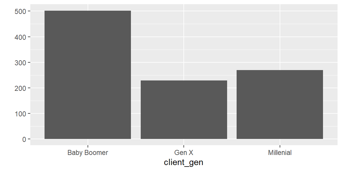
7 7 Gen XThe sample function is quite flexible and we can tweak the prob parameter, for example to say that we want (approximately) half of the population to be Baby Boomers. The effect will be visible if we produce larger amounts of data.
client_gen <- sample(c("Millenial","Gen X","Baby Boomer"), 1000, replace=TRUE, prob=c(0.25,0.25,0.5))

qplot(client_gen)
Numerical variables
The same sample() function works with numbers.
client_age <- sample(1:100,size=7,replace=TRUE)

data.frame(id=1:7,client_age)
  id client_age
1  1          4
2  2         42
3  3         33
4  4         62
5  5         76
6  6         65
7  7         81
In both cases above, each number had the same probability of being selected. If we would like some numbers to be more likely to be selected, we can specify this with prob.
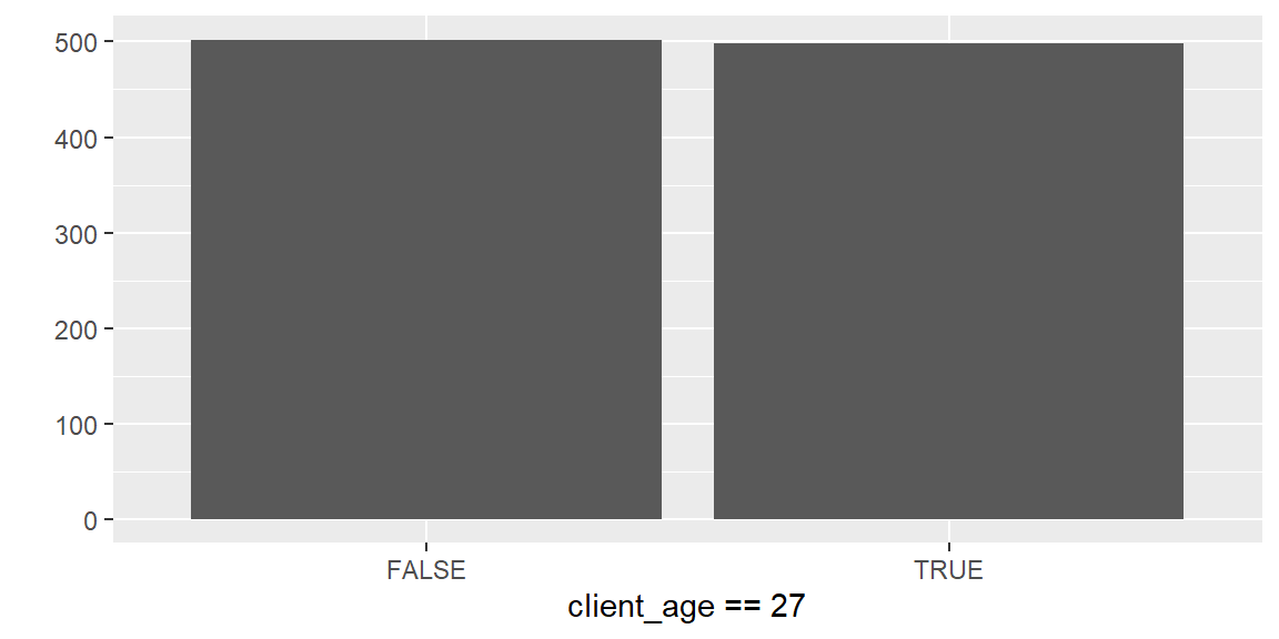
The probability values will be automatically scaled to 1. If I would like to have 50% of the population to have the age of 27, I can specify the weight. (Note: rep(1,5) is equivalent to c(1,1,1,1,1), replicating the number 1 five times.)
client_age <- sample(1:100,size=1000,replace=TRUE,prob=c(rep(1,26),99,rep(1,73)))

qplot(client_age==27)
Distributions
If you would like to work with probability distributions to create numerical variable, this is also very easy with the base functions of type r+(starting letters of the distribution).
Let’s try the uniform distribution:
client_age <- runif(7,min=1,max=100)

data.frame(id=1:7,client_age)
  id client_age
1  1   55.10342
2  2   85.19588
3  3   86.47791
4  4   73.91516
5  5   48.15197
6  6   32.90848
7  7   58.76874
As we are simulating ages, we are not interested in decimal values. We can use the round() function to round each number to the next integer.
[1] 93 26 28 29 90 81 95 3 21 62But uniformly distributed variables are not always what we want. In the example above we simulated 10,000 clients and distributes their ages uniformly. For most applications it would be unrealistic that there are as many 99 year old clients as there are 50 year old clients.
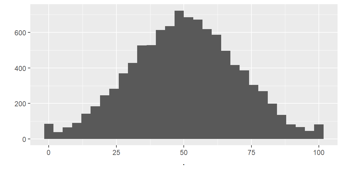
But we can easily access a whole list of other distribution functions, like the famous Normal distribution (with mean and standard deviation as parameters).
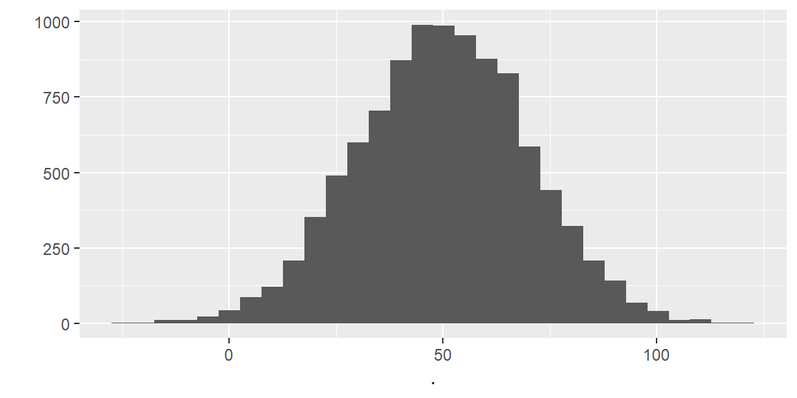
If we want to limit the values to not be smaller than 0 or larger than 100, we can use pmin and pmax.
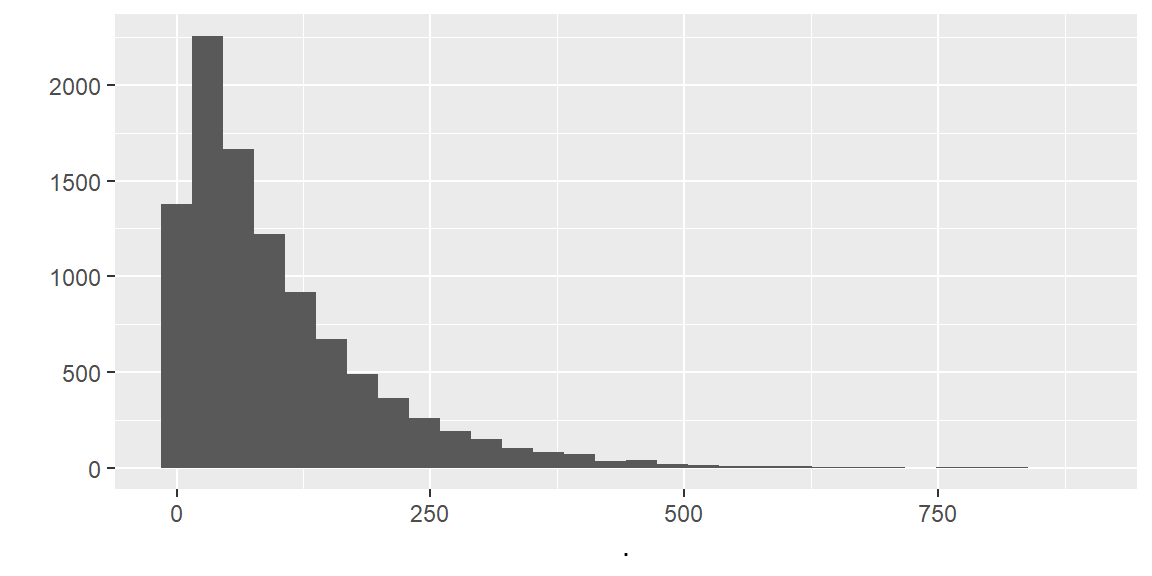
For many applications (like balance distribution or any data that contains outliers) I like to use the Exponential distribution (with parameter rate and expectation 1/rate).
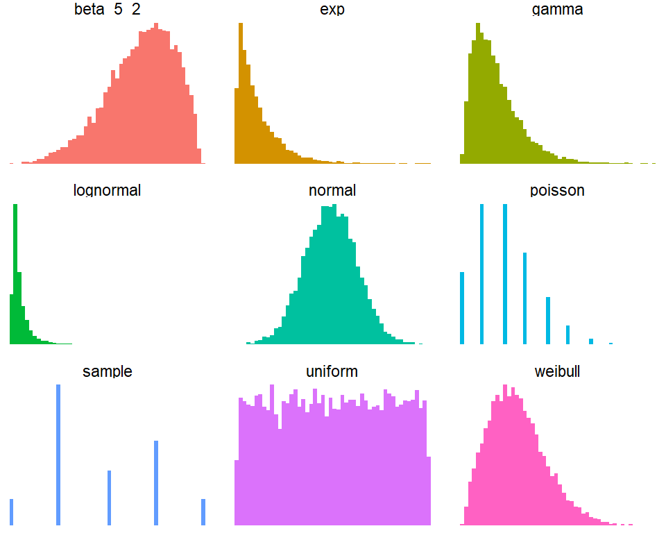
If you want to explore further probability distributions check out this link. Playing around with the parameters of the distributions you will notice that you can simulate almost any variable you like (Take a short look at: The different faces of the Beta distribution).
Combining variables in a dataframe
To create our first simulated dataframe, we can start by simulating the variables separately and then putting them together.
set.seed(61)

k <- 7

id <- 1:k
name <- c("Frank","Dorian","Eva","Elena","Andy","Barbara","Yvonne")
age <- rnorm(k,mean=30,sd=10) %>% pmax(18) %>% round()
ocupation <- sample(c("analyst","manager","sr analyst"),k,replace=T,prob=c(10,2,3))
balance <- rexp(k,rate=0.001) %>% round(2)
married <- sample(c("Yes","No"),k,replace=T,prob=c(0.6,0.4))

data <- data.frame(client_id=id,name,age,ocupation,balance,married_flg=married)
data
  client_id    name age  ocupation balance married_flg
1         1   Frank  26 sr analyst  245.96          No
2         2  Dorian  26    analyst 2273.39          No
3         3     Eva  18    manager 2270.47          No
4         4   Elena  34    analyst  373.45          No
5         5    Andy  18    analyst  961.21         Yes
6         6 Barbara  28    analyst   69.32         Yes
7         7  Yvonne  37    analyst 3218.13         Yes
Great! We just simulated a dataset which we can use now for visualization or modeling purposes.